Synchronization of rhythm in human human, human machine and machine machine interactions
Note, this is a work in progress, like a diary to formulate our thoughts and collect ideas, questions, hypothesis and results as we work towards gaining insight to the topic.
[collaborators: Johannes Fritzsche, Dimitris Prousalis, Lucas Wetzel]
We want to thank Chris Chafe and Nolan Lem for the inspiration to start this project, their shared interest and the discussions. Also note that the work discussed is based on the ideas presented in these publications:
The first two publications by Chafe and Roman study synchronization of rhythms in human interactions. Chafe et al. ask at which interaction time delay two performers achieve the best synchronization. Their results indicate that for natural time delays their synchronization works best, i.e., they are in phase and keep the frequency stable. This regime is associated to the traveling times of sound waves over distances at the scale of groups of humans.
Roman et al. tested whether a dynamical system (Stuart Landau oscillators) can reproduce the patterns observed in human synchronization. That includes phenomena like the anticipation tendency.
Shahal et al. study the synchronization between violin players while controlling the network topology, the coupling strength and the time delays (latencies) with which the players hear each other. They show that players tune their frequencies and can ignore inputs to be able to find a stable synchronized solution with others. The measurements are carried out while the time delay between the players is increased. They discuss how the observed dynamics compare to the results of a first order delayed Kuramoto model with an additional complex term that represents a bandwidth factor.
Introduction
In this project we plan to build an experimental setup inspired by the setup in Chafe et al. 2010. In our case we will use buttons instead of clapping and focus on transmission time delays (latencies) much larger than the ms presented in Chafe et al. 2010. We aim at studying human human and human machine synchronization at delays that are of the order of the period of the phrase or rhythm, i.e., s at bpm. Moreover, we can also use the setup to study machine to machine synchronization. This can be used to implement experimental setups with digital oscillators that only change their frequency at discrete instances in time, more specifically when there is an edge event at their output when the signal changes from high to low or vice versa.
The main scenarios that we will focus on first are:
I) the human to human synchronization dynamics in the presence of time delays of the order of the period of the rhythms involved, along with the question whether these can be understood and predicted by a Kuramoto model that includes signal filtering/processing and time-delayed coupling and
II) the machine to machine synchronization experiments to validate the predictions made from the analysis of an event-based dynamical model.
Experimental setup & measurements
The experimental setup is designed and build by Johannes Fritzsche – hands-on guy par excellence. He came up with the PCB design that houses two electronic drums, the microcontroller that manages delaying the trigger signals from the buttons (equivalent to the clapping buttons are tapped) by a defined time delay and sending the data to a monitoring device that stores the measurements, as well as the audio connectors and the interface to the other PCB for the exchange of the trigger signals.
First sketch of the envisioned experimental setup by Johannes Fritzsche after the initial discussions.
As can be seen in the sketch the sources of the sound are electronic drums that can be triggered by pressing a button. This trigger signal can then also be delayed artificially by a user defined value with resolution in the milliseconds regime. There are two drums on each participants side, one to play the sound triggered locally and one to play the sound of the other participant triggered with the chosen latency. The sound played by either of the drums is then mixed and played via a headphone. Depending on the type of experiment carried out the headphones are used by a human experimenter to hear is own rhythm mixed with that of the other entity, either machine or human. In the case that one or both participants of the experiment are implemented by the microcontroller, the coupling is in the simplest case realized by the exchange of the trigger signals.
Human human interaction
The rhythm to be synchronized is made by tapping a button that triggers a signal. This signal then triggers the local drum that is played to the experimenter. …to be continued…
Ising Machines
Ising Machines based on networks of mutually coupled oscillators
Note, this is a work in progress, like a diary to formulate our thoughts and collect ideas, questions, hypothesis and results as we work towards gaining insight to the topic.
[collaborators: Dimitris Prousalis, Lucas Wetzel]
We want to thank Sven Köppel and Bernd Ulmann for their shared interest and the discussions.
Introduction
This post is about our exploration into the realm of so called Ising Machines. My curiosity into the topic was sparked by discussions with genius Bernd Ulmann, Mathematician, self-appointed Analog Evangelist, Inventor, Founder, museum director and most importantly a nice person.
An Ising machine is a physical implementation of a spin-system and its interactions to compute minima of the Ising Hamiltonian. As reviewed and shown, e.g., in “Ising formulations of many NP problems” by Andrew Lucas, many NP hard problems can be mapped onto the Ising Hamiltonian. Hence, if an Ising Machine can be build and scaled, it can act as an analog computer to solve these NP hard problems by finding/relaxing to ground states of the system. (Which is not guaranteed since the system may get trapped in a local minima. In this case some “shaking may help”.)
First of all I would like to link the first publications that I read to start with the topic. To be honest, they gave me a bit of a headache since by no means I was able to confirm the results that they presented when I stared looking at them in early 2021 — but more on that later. Here is the list to the open access manuscripts:
When scaling Ising Machines to large numbers of spins (represented by oscillators whose phases are binarized) and to operate at high frequencies, the systems (spatial) dimensions may lead to non-negligible transmission time delays in the connections between the oscillators. We know, that such time delays can lead to multistability of in- and anti-phase synchronized states and therein. Furthermore, as the problem is usually encoded via the adjacency matrix of the network, these time delays will most likely be heterogeneous. Also, it has been shown that inert responses in, e.g., electronic oscillators, that stem from signal processing affect the self-organized dynamics in such systems.
The question is then, whether the mapping to the Ising Hamiltonian can still be justified and if not, which measures can be taken to achieve a sufficient (to solve a problem) approximation. TODO: compile a list of open questions and problems related to the presence of time delayed coupling and inertia, quantify their effects in simulations and look for ways to address these.
When simulating delay-coupled phase oscillators using the Kuramoto model we made the following observations:
a) The results in Oscillator-based Ising Machine, chapter IV: Examples can be reproduced for sufficiently strong dynamical noise. If the noise was too small, we did not observe the convergence to the correct MAX-CUT solutions in all cases (actually we observed that only rarely). This could be a sign for rugged energy landscapes that require some ‘shaking’ to find the absolute minima and hence the correct solutions to the MAX-CUT problem.
b) When simulating using a second order Kuramoto model that takes into account inertia like effects introduced by, e.g., a loop filter in a phase-locked loop or the mass of a pendulum, the phases did not converge to the correct solutions for arbitrary loop filter cut-off frequencies. Increasing the cut-off frequency, or in other words, reducing the oscillators inert behavior, led again to the correct solutions. My hypothesis is, that loop filters with cut-off frequencies far below the second harmonic injection frequency will damped this too strongly and prevent he binarization of the oscillators phases. Hence, it may be beneficial to mix the second harmonic injection locking signal directly into the control signal of the PLL. In principle it may be possible to use a ‘copy’ of the feedback signal which is mixed with itself. The resulting output can then be filtered by a band-pass that allows only the second harmonic. These are however details the implementation of such an idea, in e.g., a PLL type of setup.
c) Adding small transmission delays seemed not to hinder convergence to the correct solutions, independently of whether the time delay would have led to in- or anti-phase synchronized states.
Notes for publication:
issues to be addressed: subharmonic injection locking in the presence of transmission delays that affect the frequencies of the oscillators – in that case the injection locking has to happen at roughly twice the instantaneous frequency of the oscillators
approaches discussed so far in the literature with electronic oscillators:
a) T. P. Xiao, Optoelectronics for refrigeration and analog circuits for combinatorial optimization, Ph.D. thesis, UC Berkeley (2019).
b) relaxation oscillators with capacitive coupling: A. Parihar, N. Shukla, M. Jerry, S. Datta, and A. Raychowdhury, Scientific reports 7, 1 (2017).
c) CMOS LC oscillators on chimera graph: N=240 in T. Wang, L. Wu, and J. Roychowdhury, in Proceedings of the 56th Annual Design Automation Conference 2019 (2019) pp. 1–2. and N=5 in J. Chou, S. Bramhavar, S. Ghosh, and W. Herzog, Scientific reports 9, 1 (2019).
d) RLC oscillators: LQ English, A. V. Zampetaki, K. P. Kalinin, N. G. Berloff, P. G. Kevrekidis, arXiv preprint arXiv:2204.00153
Playground, simulations & observations
Here I collect some results obtained from simulating different types of Kuramoto models. The code used here can be found on Github. The documentation process is still underway and I am being supported in cleaning up and organizing the code by Deborah Schmidt.
Along the results presented in Oscillator-based Ising Machine obtained by Matlab simulations of the Kuramoto model we start here and ask whether these results can be reproduced. Our model reads in the most general form [1,2,3]:
(1)
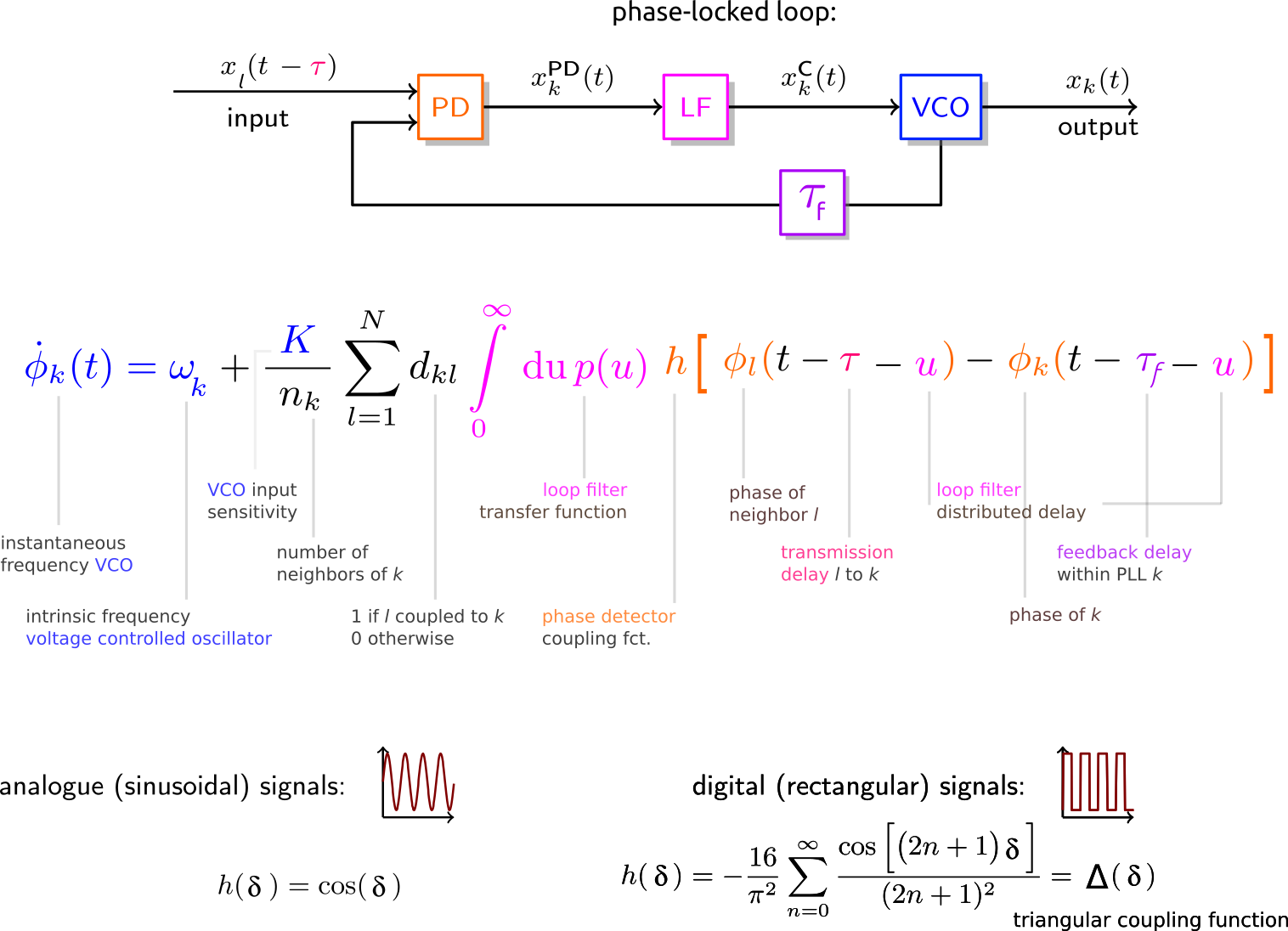
where denotes the instantaneous frequency, and the intrinsic frequency of oscillator , with . denotes the coupling strength or sensitivity towards input signals to oscillator from other oscillators in the network, as given by , the components of the adjacency matrix that are either one or zero depending on whether there is a connection from oscillator to or not, respectively. The integral represents the signal processing or filtering within the feed-forward path of the oscillators, e.g., a low pass filter in a phase-locked loop oscillator with impulse response function . denotes the phase of oscillator , the transmission time delay for signals propagating from oscillator to , and the feedback time delay within oscillator . denotes the strength of the harmonic injection locking. Finally, denotes additive Gaussian white noise with variance .
In terms of the model, we aim to address how the following parameters affect finding the ground states and relate to the classical Ising model:
how to appropriately increase or , which one preferably and at what rate, does it depend on the network size?
the role of the loop filter via the , the filter transfer function – if the cut-off frequency is below the harmonic frequency, then the injection locking signal will be damped/filtered and binarization may be impaired (here we should consider a modified PLL architecture where the harmonic injected signal does not pass trough the loop filter, e.g., multiplication by itself and band-pass to extract harmonic)
the role of feedback and transmission time delays, as the size of a system grows it becomes increasingly difficult to arrange the oscillators such that they can be coupled to any other in the network with the same transmission time delay; question: if there are transmission time delays that are heterogeneous within one connection (asymmetric), i.e., between an oscillator and and oscillator , this leads to phase-difference between these oscillators for the case of pure mutual coupling without injection locking – how does that affect a networks ability to relax to a ground state of the Ising model? the same holds for the case and
what about the coupling capacity/normalization of the inputs? does an oscillator couple more strongly the more inputs it receives?
should the coupling between the oscillators be repelling, i.e., should ?
Reproduce
When removing the loop filter , for zero time delays , for identical oscillators , and for independently of the number of inputs we find
(2)
In the publication Oscillator-based Ising Machine, see chapter IV, they set radHz, radHz and simulate different network topologies, using simple MAX-CUT problems to benchmark. Note, that here the coupling strength is increased linearly / ramped up once the simulation has started. We chose for the noise strength (radHz).
Using the same parameters we find the following results for a system of oscillators, where oscillator receives input from all other oscillators while all other only receive from oscillator . Hence, we have a star-like topology with oscillator being the center. In this case, the MAX-CUT problem is solved if all oscillators evolve to a phase different by from that of oscillator . The results were promising and lead to the correct solution of the MAX-CUT problem in most cases, however not in all cases as we show in the figures below:
(correct solution)
Fig. 1: Shows the frequency of all oscillators in the first row, the phase differences with respect to the phase of oscillator k=1 (dashed line) in the second row and the Kuramoto order parameter in the third row. Observe how the binarized phases of the oscillators separate successfully the nodes of the network into two groups according to the MAX-CUT of this network.
(incorrect solution)
Fig. 2: Shows the same plots as in Fig. 1 above. Observe how a few of the binarized phases of the oscillators do not separate to the correct subgroup and hence the MAX-CUT problem was not solved correctly. In this case we may have ramped up the coupling strength too quickly. This is an aspect that we will explore in more detail in the following.
We then realized the importance of the process of ramping up the coupling strength for finding the correct solution successfully. Also, adding dynamical frequency noise seemed to help convergence. Moreover, we simulated some realizations with time delay, signal filtering and ramping up the harmonic injection coupling strength instead of the coupling strength of the first harmonic coupling terms. This had profound impact on whether the correct solution to the optimization problem was found. Therefore we decided to develop ideas on how to approach the impact of these parameters in a more structured way. Our preliminary results is what we will present in the following.
How we measure the success probability and time to solution as we change different system parameters?
We decided to run a number of realization for a fixed set of parameters and solve the MAX-CUT problem for a system of oscillators arranged in a star like topology, where an oscillator indexed by is located in the middle of the star and hence receives input from all others, while all others only receive input from , the center oscillator. After computing realizations we ask how many have led to a correct solution and in what average time that was achieved. A realization is categorized at being solved correctly when the magnitude of the order parameter settles at a value of in that particular case, i.e., all phases have separated correctly. The Kuramoto order parameter is defined as
(3)
where denotes the magnitude of the order parameter and the mean phase. measures the synchrony of the oscillators and approaches if all oscillators are in-phase. In our benchmark case, all outer oscillators of the star topology form a subset that is shifted by a phase difference of with respect to oscillator . One can then calculate
(4)
which yields the result for the particular MAX-CUT problem used for benchmarking here mentioned above and visible in Fig.~1.
A few more words on how we obtained the statistics on the realizations automatically from the simulations.
In order to determine whether the correct solution to MAX-CUT problem was found we checked the asymptotic values of the phase differences. Hence, if the phase differences of all oscillators with respect to the phase of are equal to asymptotically, the correct solution has been obtained. We quantify this by checking these phase-differences and the value of the order parameter. Since the phase-configuration should be constant once the system has settled to the ground state, we compute the average over one and a half period of the intrinsic oscillations of the oscillators.
Extracting the mean time until a solution is obtained is measured as follows. We consider only those realizations that led to a correct solution of the MAX-CUT problem. For these, we calculate the time-derivative of the order parameter which we then average over half a period of the intrinsic frequency of the oscillators. This yields a more smooth curve. We then track from the end of the time-series towards the beginning, i.e., backwards in time, when the order parameter changes for the first time. This represents the end of the transient dynamics that led to the solution. To calculate the time to solution, we choose the difference between the time when the transient dynamics have finished and the time where we started to ramp up the coupling strength.
Here is an example how the resulting plots look like:
Fig. 3: Kuramoto order parameters for all 18 realizations as a function of time in one plot. The blue dots at R(t)=0 mark the points between which we measure the time to solution for correct solutions. The text box shows the statistics, i.e., the percentage of realizations that led to the correct solution and the average time that this required.Fig. 4: All Kuramoto order parameters (blue) and their time derivative (red) for all realizations as a function of time in individual plots. The blue dots at R(t)=0 mark the points between which we measure the time to solution for correct solutions. The text box shows the asymptotic value of the order parameter.Fig. 5: Time series of all phase differences with respect to the phase of oscillator k=1 (dashed line). Initially the phases were distributed between -pi and pi, here they are plotted between -pi/2 to 3pi/2. In that case in- and anti-phase synced states are clearly visible without noise induced slips at the modulo boundary. All realizations show the correct solution to the MAX-CUT problem.Fig. 6: Time series of the output signals of all oscillators, here digital, plotted for each realization individually.
Results for networks of oscillators that respond instantaneously and where no transmission time delays are present
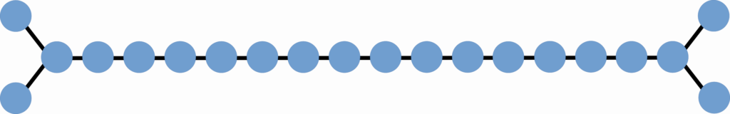
In a network of mutually coupled oscillators with second harmonic injection locking (SHIL) we show that the Maximum cut problem can be reliably solved. The oscillators have an infinite modulation bandwidth and there are not time delays associated to the mutual coupling between the oscillator nodes of the network. We benchmark with the network topology shown in Fig. 7.
Fig. 7: Network topology used to benchmark the MAX cut problem with equal edge weights.
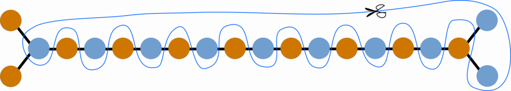
The correct MAX cut solution to this problem looks as shown in Fig. 8, where the different colors separate the two populations of nodes defined by the Maximum cut.
Fig. 8: Maximum cut solution to the network topology shown in Fig. 7.
The result of the realizations shown in the plots were obtained for random initial conditions, choosing the initial phases of all oscillators as independent and identically distributed random variables from the interval . For some initial time we simulate the oscillators dynamics in the presence of noise and the SHIL perturbation with constant radHz. Then we ramp up the coupling strength of the mutual interaction terms from radHz to radHz, as shown in Fig. 9.
Fig. 9: Time dependence of coupling strength of the mutual coupling between the oscillators in Hz/[Volt].Given the ‘ground truth’ above, we hence expect that oscillators align to one group and the other to the group that is separated by from the first. The order parameter is then expected to be equal to zero. Here we show the plots of the phase differences with respect to the first oscillator in the system, see Fig. 10. Note that in the plots the oscillator numbering starts from and ends at .
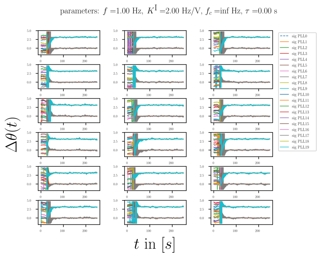
Fig. 10: Phase differences of all oscillators with respect to oscillator . After free-running for few cycles the noisy oscillators with SHIL are coupled by linearly increasing the coupling strength , see Fig. 9 and two populations with distinct phase differences form.
The order parameter plots associated to the phase difference plots in Fig. 10 reveal that there are indeed two populations with oscillators in each. The populations are separated by a phase-difference and hence the order parameter , see Fig. 11.
Fig. 11: The order parameter (blue) and its time derivative (red) as a function of time. The final (mean) value of the order parameter is specified in the legend for each realization. The cyan diamonds represent the beginning and end of the measurement that is dedicated to measuring the time to solution.
An overview plot of all the order parameters for all realizations and the ‘statistics’ (it’s only 18 realizations) concludes that all cases were solved correctly by the relaxation dynamics, see Fig. 12. Note that the automatized measurement of the relaxation time, i.e., the time to solution failed here due to the fluctuations of the order parameter. This feature will be reworked in the next iteration.
Fig. 12: All order parameters for all realizations. Note that due to the fluctuations of the order parameter the automatic estimation of the time to solution FAILED. From inspection by eye we estimate an average time to solution of about 30-50 periods of the intrinsic frequency.
Hence we have to rework the way the automatic estimation of the time to solution is performed. We will use smoothing functions in the future to obtain a moving average that accounts for boundary effects. These results show that with the right choice of parameters , , and , the slope of the linear ramp the network of mutually coupled oscillators solves the Maximum cut problem correctly with probability one.
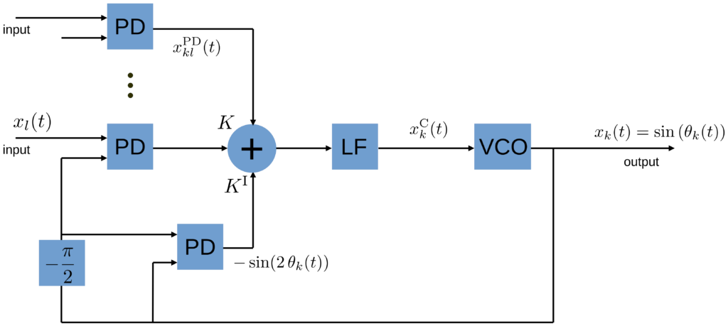
The results shown so far correspond to the following architecture design schematic of an oscillator with SHIL, see next Fig. XY.
Fig. XY: Schematic of a PLL with SHIL. There are no time delays in the network.
Adding inert oscillator responses
In that case we obtain the following set of dynamical equations
(5)
where the same notation holds as provided following Eq. (1). Note that in the case presented here, the SHIL signal is also filtered by the LF that filters the cross-coupling signals between the oscillators, see schematic Fig. XY1. This is an architecture design choice. We will later also discuss the case where the SHIL signal is added after the LF and is not filtered by the low pass.
Fig. XY1: Schematic of a PLL with SHIL. The SHIL signal and the cross-coupling signals are filtered by the low-pass filter (LF).
Adding inert oscillator responses and transmission time delay
In that case we obtain the following set of dynamical equations
(6)
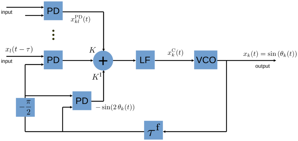
where the same notation holds as provided following Eq. (1). Note that also in the case presented here, the SHIL signal is also filtered by the LF that filters the cross-coupling signals between the oscillators, see schematic Fig. XY2. This is an architecture design choice. We will later also discuss the case where the SHIL signal is added after the LF and is not filtered by the low pass.
Fig. XY2: Schematic of a PLL with SHIL. The SHIL signal and the cross-coupling signals are filtered by the low-pass filter (LF). The external signals and the feedback signal can be time-delayed.
Inert oscillator responses, transmission time delay and no LF filtering of the SHIL signal
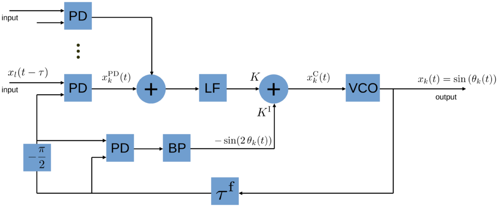
In this case the SHIL signal is not fed through the LF together with the cross-coupling signals, however instead there is a band-pass filter that ensures that only the second harmonic contributions from the self-mixing of the oscillators passes to the control signal, see Fig. XY3.
Fig. XY3: Schematic of a PLL with SHIL. The SHIL signal filtered by the band-pass filter (BP), while the cross-coupling signals are filtered by the low-pass filter (LF).
Control theory of mutual synchronization in networks of delay-coupled phase-locked loops
This post is related to a manuscript that we have submitted for publication to IEEE Access and I will extend this summary here step by step.
Introduction
In classical phase-locked loop (PLL) theory concepts like the gain and phase margin and application of the Nyquist criterion help to analyze the stability of a system. These are accessed from the PLLs transfer function in Laplace space and analysis at the critical point for zero real part of the Laplace variable. Hence, the stability of the system is studied where it changes from stable to unstable, in dynamical systems theory we call this the marginal stable case. At this point, the above mentioned concepts rely on the variation of the complex part of the Laplace variable, the frequency. From this, Bode and Nyquist plots are constructed and gain and phase margins defined.
This is straightforward for the case of the entrainment of a PLL by a periodic reference signal. However, in the literature on classical PLL theory one aspect is often missing — the effect of the synchronized or entrained state itself. Here, I will discuss this topic and show how the transfer functions of PLLs and networks of PLLs change because of it.
On the differences between universal emergent time (UEC) and universal coordinated time (UTC)
This is to become a collection of thoughts on the future of self-organized synchronization in coordination and timing applications. On the one hand it will be a collection of the current applications that I see as a potential use cases and markets, on the other hand I will continue the process of boiling down the differences of this approach to state-of-the-art hierarchical solutions. The concept of a spatially distributed emergent clock vs the concept of many individual clocks that are spatially distributed and corrected in a hierarchical manner will be discussed. Also, I am happy for any criticism, feedback and thoughts.
WORK IN PROGRESS
This is supposed to be more a basis for discussion and thought than a source of factual information.
State-of-the-art time-standards based on reference periodic processes
A time standard is a specification on how to measure time which historically were often bound to Earth’s rotational period. Time standards provide either a way to specify how fast time passes, and/or provides fixed points in time.
The current time-standards important for most of our everyday life are the coordinated universal time (UTC) and the international atomic time (TAI). For those who wonder about the order of letters in the abbreviations have their origin in french, i.e., temps atomique international and temps universel coordonné. While UTC is organized to stay close to mean solar time, it is related to the TAI time standard which is tied to the definition of the SI second.
So far most of the existing time-standards are related to a reference, such as the periodicity of the Earths rotation or frequencies related to physical processes. Subsequently other clocks can be synchronized to the time defined by these standards in a hierarchical way. This of course relies on the transmission of signals for the correction of time within the network of spatially distributed clocks. At large distances and/or high frequencies this become a challenging part, even if the signal transmission times can in general be measured and compensated for. The quality of synchronization then depends on the accuracy with which the signalling times can be measured.
In summary that means, that synchronization via hierarchical solutions relies on very frequency stable reference clocks that feed-forward their signal to individual distributed clocks in order to correct the time-deviations arising due to the inevitable (there are no identical clocks) drift.
I would like to note there, that the TAI is not a hierarchically synchronized systems but instead a plesiosynchronous system. There is no coupling between these clocks. However, their difference towards their weighted average is used to correct the time-stamps that they provide to third parties. The plesiosynchronous approach is usually chosen for networks that consist of very frequency stable clocks/oscillators.
A time-standard based on a spatially distributed clock arising over a network of mutually delay-coupled clocks
Howto run independent voltage noise sources (IID and GWN) in LTSpice using Bv-sources
In order to have two independent noise sources with a different random seed the rand(), or random(), or white() LTSpice-functions have to be called with a different argument, e.g.:
Generate Gaussian white noise (GWN) distributed pseudo random numbers from independent identically distributed (IID) random numbers using the Box-Muller transform:
,
with mean and standard deviation . Note, that the two iid pseudo random numbers generated using the LTSpice rand()-function have to have different seed.
As soon as I find the time I will check how well that works in LTSpice and provide plots and statistics. Any feedback is very welcome.
Spice simulation of self-organized synchronization with LTC6900 oscillators
LTspice based simulations of mutually delay-coupled digital phase-locked loops (DPLLs) using an LTC6900 oscillator as a VCO. These simulations take into account the dynamics of the voltages and currents, as well as the processing time of different electronic circuitry used in PLL components. The circuitry aims at testing the control of self-organized synchronization in such networks, starting with a minimal system. We compare the results to our theoretical predictions of a phase-model.
This is work in progress, give us feedback!
We use LTspice, an open source analog circuit simulator to simulate systems of coupled DPLL on the level of the voltage and current time-series. Using this industry-standard approach to test the circuit architectures down to the transistor level before setting up the prototype systems for experimentation allows to identify potential problems such as parasitic resistances and capacitances. We also use it to gain a better intuition on the dynamics within the circuitry as components become heterogeneous and are subject to noise.
Here we present our current ongoing work on a system of mutually delay-coupled digital phase-locked loops (DPLLs), each consisting of a phase detector (here XOR), a loop filter (first order RC-filter low pass) and a voltage-controlled oscillator (VCO), specifically the LTC6900 model from Analog Devices.
We couple these DPLLs with each other and without a time reference and consider signal transmission, feedback and processing delays in the network and the nodes. The concept behind this setup is a publications in PLOS ONE and the New Journal of Physics, titled Self-organized synchronization of digital phase-locked loops with delayed coupling intheory and experiment and Synchronization in networks of mutually delay-coupled phase-locked loops. In these publications the frequencies and phase configurations of self-organized synchronized states and their stability are analyzed for networks of analog and digital phase-locked loops using a phase model. In such networks different types of synchronized states exist, for which the frequencies of all PLLs can adjust to a common global frequency in a non-linear dependence on the time-delays and the coupling strengths, while different phase configurations are possible. These states with the different phase configurations are called splay or m-twist synchronized states. Whether such states are stable strongly depends on the transmission-delay between the oscillators, the coupling strength and the internal process of the oscillator nodes, such as signal filtering and feedback delay-times.
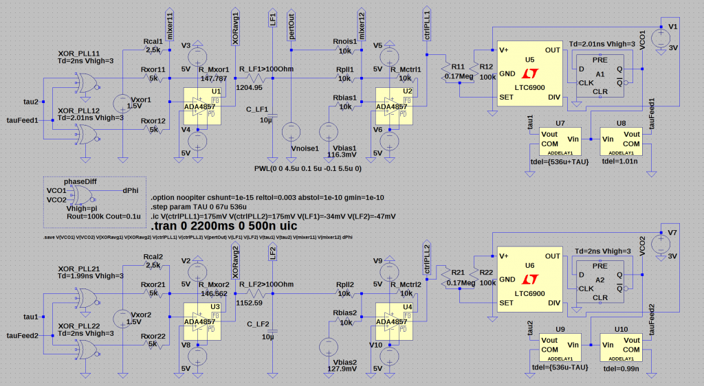
LTspice block level circuit diagram of two delay-coupled DPLLs
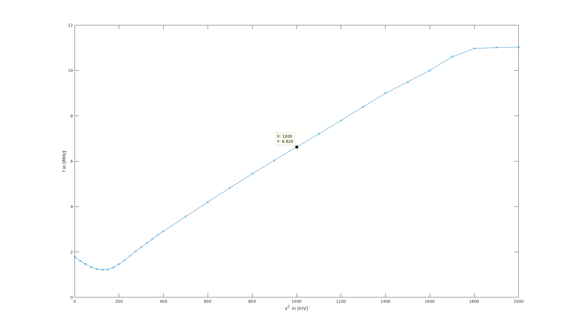
We start with a system of mutually delay-coupled DPLL clocks running at a mean intrinsic frequency of MHz, see Fig. 1: LTspice block level circuit diagram of two delay-coupled DPLLs. Before that, we perform a separate SPICE simulation to measure the input response of the voltage-controlled oscillator, in this case a LTC6900, of our DPLLs. Hence we perform a parameter sweep transient simulations for each of which we change the input voltage to the LTC6900 VCO and measure the frequency of the output signal. We obtain the frequency from a Fourier analysis, using the FFT tool of the LTspice software. The result is shown in Fig. 2: VCO response curve. Note that we use a d-flip-flop at the output of the LTC6900 that divides the frequency by a factor two and ensures a duty cycle of 50%.
Fig. 2: Frequency response curve of LTC6900.
The slope of the linear fit is the input sensitivity of the VCO with MHz/V and the free running frequency MHz. As can be seen from the circuit diagram, the output signals of the two (here redundant) XOR phase detectors are mixed together with a shift voltage . The mixer is designed such that it takes into account all XOR outputs, that potentially originate from different coupling pairs, equally. makes the center frequency of the full setup adjustable and sets the operation point. This part is followed by the loop filter, here a first order RC low pass, whose output is fed into a second mixer that combines the offset signal . The offset signal can also shift the center frequency of the VCO, as will become clearer in the following. In the next step, we establish how the parameters of the SPICE circuit level simulations translate to the parameters of the phase model. With this we bridge the gap between these two abstraction layers. The phase model reads
(1)
where indexes the PLLs in the network, denotes the instantaneous frequency, the intrinsic frequency, the coupling strength, the number of input signals to PLL , the impulse response of the loop filter, the transmission-delay of a transmission delay line between nodes and , the feedback delay-time in the feedback path within PLL to the input of PLL , and the are either one or zero, depending on whether there is a connection or not. The parameters of the phase model have the following connection to the parameters of the LTspice circuit simulation
(2)
where denotes the intrinsic frequency in the phase model and the coupling strength, of the XOR output, and the scaling factor that scales the input sensitivity . In the circuitry this scaling is implemented by a closed-loop operational amplifier (here inverting) that measures voltage differences at its (high impedance) input and outputs the this voltage amplified with an amplification factor given by the relation of the resistors and .
Spice simulations of digital phase-locked loop systems
LTSpice based simulations of two mutually delay-coupled digital phase-locked loops (DPLLs). These simulations take into account the dynamics of the voltages and currents, as well as the processing time of different electronic circuitry used in PLL components. We compare the results to our theoretical predictions from the phase-model.
We use LTSpice, an open source analog circuit simulator to simulate systems of coupled DPLL on the level of the voltage and current time-series.
Using this industry-standard approach to test the circuit architectures down to the transistor level before setting up the prototype systems for experimentation allows to identify potential problems such as parasitic resistances and capacitances. We also use it to gain a better intuition on the dynamics within the circuitry as components become heterogeneous and are subject to noise.
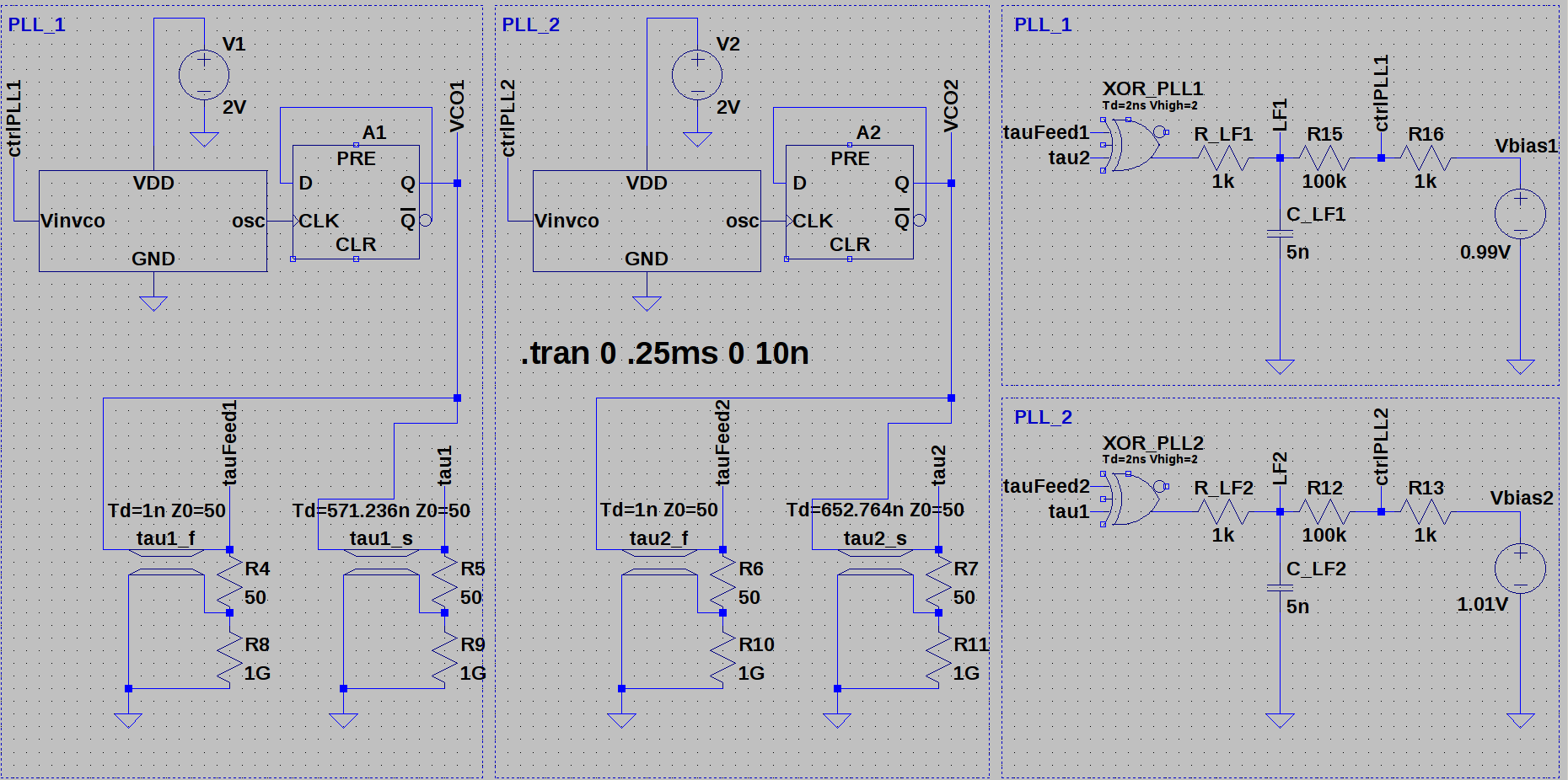
Here we present our current ongoing work on a system of two mutually delay-coupled digital phase-locked loops (DPLLs), each consisting of a phase detector (XOR or flip-flop), a loop filter (first order low pass filter) and an voltage-controlled oscillator (VCO). The VCO is a ring oscillator which is set up from a closed chain of inverter elements, designed by Jacob Baker and available from YOUSPICE.
Fig.1: Two digital phase-locked loops with first order loop filter, delayed feedback and transmission lines for mutual coupling. The DPLLs are separated into two part, the VCO and delay-lines (left), and the phase-detector and loop filter components (right). No reference clock involved.
Before going into the details of this circuit, we show the response curve of the VCO plotted against the input voltage at Vinvco.The VCO is supplied by a 2V power source and we changed the parasitic capacitor in the inverter subcircuits of the VCO to fF.
Fig. 2: VCO with rectangular output signals designed by R. Jacob Baker. The measurements are included as a table.
Fig. 3: Response curve of VCO (ring oscillator) for supply voltage 2V and parasitic capacitance .
Science Slam @Elbhangfest in Dresden, 2018/06/23
This is the guiding draft for a Science Slam that I contributed at the Elbhangfest 2018 in Dresden.
In the beautiful scenery of Pillnitz Palace at the riverside of the Elbe, the stage hosted great contributions from the Arts, Music and Science in a thoughtful mix.
(deutsche Fassung weiter unten)
Simultaneity. On synchronization in modern electronic clocks.
I would like to start with an experiment. Please applaud now, as if you all wanted an encore from your favorite band.
[wait until the audience has found a common rhythm of clapping their hands]
As you probably heard, it took a while until you had found a common rhythm. This rhythm was self-organized, as each of you adjusted the repetition speed of clapping according to that of your neighbors. In other situation, e.g., in large soccer arenas synchronizing is much harder. This is because of the relatively large distances and the delay with with each person perceives the clapping of distant fans.
[short pause]
Now imagine, hundreds or thousands of elements, e.g., electronic clocks need to be coordinated in time. And those do not “clap” just once, but tick many billions of times in a second. Currently, this coordination is achieved by a precise reference clock that dictates its time to all other clocks. That means: a conductor, placed well visible in the middle of the arena, provides the rhythm for a billion claps per second to the audience. That of course impossible thing for the conductor, also reaches its limits in electronic systems.
[short pause]
Looking for alternatives, we were inspired by work from colleagues at the Max Planck Institute for Molecular Cell Biology and Genetics. They study the astonishing periodicity of the formation of the vertebrae during embryonic development. The rhythm necessary for that pattern formation results tissue-wide by the interactions of hundreds of cellular clocks. That also works in the presence of large time-delays in the intercellular communication. That means, similarly to how you as a group found a common rhythm, the cells self-organize their mutual states to be the same.
[short pause]
We formalized this approach to coordination without a dictating conductor in an abstract mathematical model. That helped us to understand how to transfer the concept of self-organized synchronization in the presence of time-delayed communication to electronic systems. Experiments in prototype systems show promising results and great agreement with the model. Our goal is to apply this approach in modern technologies, such as e.g. indoor navigation and robotics. Moreover, we aim to enable new technologies that could not be realized with the hierarchal approach.
Thank you for your attention.
Was bedeutet gleichzeitig? Über die Synchronisation moderner Uhren.
Ich möchte mit einem Experiment beginnen. Bitte applaudieren Sie jetzt alle so, wie sie es tun um eine Zugabe bei einem Konzert Ihrer Lieblingsband zu bekommen.
[warten bis das Publikum einen gemeinsamen Rhythmus gefunden hat]
Wie Sie hörten dauerte es eine Weile bis Sie einen gemeinsamen Rhythmus gefunden hatten. Diesen haben Sie als Gruppe selbst organisiert indem Sie ihr Klatschen an das Ihrer Nachbarn angepasst haben. In anderen Situationen, z.B. im (Fussball-)Stadion wäre das schwieriger. Grund dafür sind die relativ großen Entfernungen und die Verzögerung mit der Sie das Klatschen von weit entfernten Besuchern wahrnehmen.
[kurze Pause]
Nun stellen Sie sich vor, es müssen hunderte oder tausende von Einheiten, z.B. elektronischen Uhren zeitlich aufeinander abgestimmt werden. Und diese “klatschen” nicht wie wir nur einmal, sondern ticken 1 Millarde mal pro Sekunde. Bisher wird diese Koordination durch einen präzisen Taktgeber der allen anderen Uhren die Zeit vorgibt realisiert.
Heißt: in der Stadionmitte steht ein Dirigent und gibt den Milliarden-takt für alle gut sichtbar an. Was für unseren Dirigenten unmöglich ist führt auch die elektronischen Systeme an die Grenzen des Machbaren.
[kurze Pause]
Auf der Suche nach Lösungen, die diese Hürden überwinden können, haben wir uns von unseren Kollegen am Max Planck Institut für molekulare Zell- biologie und Genetik inspirieren lassen. Sie beschäftigen sich mit der zeitlich streng koordinierten Formation der Wirbelkörper während der embryonalen Entwicklung. Der dafür notwendige Rhythmus ergibt sich gewebeübergreifend aus dem Zusammenspiel hunderter von individuellen zellulären Uhren. Das funktioniert auch dann, wenn die Kommunikation einer großen Zeitverzögerung unterliegt.
Das bedeutet also, in ähnlicher Weise wie Sie zu Beginn einen gemein-samen Rhythmus gefunden haben, selbst organisieren die beteiligten Zellen ihre Zustände.
[kurze Pause]
Diesen Ansatz der Koordination ohne taktvorgebenden Dirigenten haben wir in einem abstrakten mathematischen Modell formuliert. Damit haben wir verstanden wie wir das Konzept der selbstorganisierten Synchronisation auf verteilte elektronische Systeme übertragen können. Experimente an Prototypen zeigen dabei vielversprechende Resultate. Unser Ziel ist es, diese Idee in modernen technologischen Anwendungen, wie z.B. der Robotik und der Innenraum-Navigation, zu etablieren und neue Anwendungen zu ermöglichen, die mit dem aktuellen Stand der Technik nicht umzusetzen sind.
Self-organized synchronization in electronic systems
[collaborators: Nirmal Punetha, Niko Joram, Suropriya Saha, Shamik Gupta, Sara Ameli Kalkouran, Josefine Asmus, Daniel Platz, Benjamin Friedrich, David J. Jörg, Alexandros Pollakis, Wolfgang Rave, Gerhard Fettweis, Frank Ellinger, Frank Jülicher]
This project started as a collaboration between the Max-Planck Institute for the Physics of Complex Systems and the Vodafone Chair Mobile Communications Systems at the TU-Dresden within the Center for Advancing Electronic Dresden. In this project we explore self-organized synchronization of mutually delay-coupled electronic clocks. This concept with a flat hierarchy is different from the State-of-the-Art hierarchical approach to synchronization, where a reference clock dictates the time to all other clocks.
In electronic systems, information processing shared between large numbers of units and in parallel has become more and more important. Prominent examples are antenna arrays in radar and mobile communications, servers and databases, networks-on-chip, indoor and global navigation solutions, swarms of drones and robots, and sensor arrays. In such systems, robust operation and processing requires coordination of the components involved. This can be achieved by a common time-reference that is provided by clocking devices. In practice it can be a challenging task to provide such a system-wide reference, given the heterogeneity of CMOS integrated circuitry, the dimensions in space or number of such systems and the frequencies of operation. The time-delays in electronic signal transmission become important when the wavelength of a signal is of the order of the spatial dimension of the system. That means, that signal transmission delays become relevant once they are of the order of the time-scales of operation of the system. For example, for electronic components that are clocked at frequencies in the GHz regime, distances of a few milli- to centimeters become important even for signal transmission at the speed of light.
Our research focuses on self-organized synchronization of electronic clocks. While the state-of-the art approach to synchronization in electronic systems uses precise reference clocks, e.g., quartz oscillators or atomic clocks to entrain many low quality electronic clocks, so called phase-locked loops, we couple the cheap low quality clocks with each other in a setup that allow for synchronized states to form self-organized over such networks. This has the advantage, that communication delays do not need to be compensated for, e.g., by constructing complicated clocks trees or measuring signal transmission times. Furthermore, dynamically changing network topologies with large numbers of elements become feasible. This would allow to synchronize systems globally instead of following the globally asynchronous locally synchronous (GALS) solutions of most of todays electronic hardware.
The MODEL — identical phase-locked loops
In this project we derived a mathematical model that is independent of the details of the circuitry of phase-locked loop (PLL) clocks. These consist of three main components, the phase-detector (PD), the loop filter (LF) and the voltage-controlled oscillator (VCO) and a signal path that feeds the output signal back to input. We start with generic periodic VCO output signals for which we assume constant amplitudes. These are exchanged between the PLLs. In each PLL, the PD detects the low and hight frequency components of the combined feedback and external input signals. Subsequently we assume, that the LF filters the high-frequency components ideally, which yields the control signal that affects the instantaneous frequency of the VCO. Under these assumptions we obtain a phase-model description of the dynamics of the instantaneous frequencies in PLL networks.
Schematic of a PLL and phase-model for a network of mutually delay-coupled PLLs.
For a Dirac-delta impulse response of the LF and no feedback and transmission delay, this reduces to the well known Kuramoto model of coupled phase-oscillators.
Synchronized solutions
From this model we can calculate the frequencies and phase relations between all oscillators in a network. In the case of identical clock elements the frequencies of synchronized states depend on the intrinsic frequencies of the individual clocks, the coupling strength, the feedback and transmission delays and the coupling function. There are also states with constant non-zero phase differences between the clocks, which are called -twist or splay states.
Linear stability
Whether these synchronized states are stable, marginally stable or unstable can be determined by performing a linear stability analysis. This requires the information about the network topology, i.e., which PLLs are coupled, the internal parameters of the clock elements and the transmission delays.
Experimental setup and results
We validated our theoretical predictions that were obtained using the phase model by carrying out experiments in prototype PLL networks. These consisted of low cost self-soldered PLLs prototypes running at kHz.
Using a microcontroller to artificially delay the coupling between PLLs at 1kHz
In order to measure the effects of transmission delay with clock elements running at just kHz, delay-times should be of the order of milliseconds and at least s. Instead of using hundreds of kilometers of copper wiring, we use a micro-controller that buffers the states and histories of the PLLs and then sends these signals at specified delays to the respective coupled nodes in the clock network.
Sketch of experimental setup of mutually delay-coupled DPLLs.
The experimental results confirm qualitatively and quantitatively the theoretical model predictions and can be found in the links to the published work at the beginning of this blog entry. In those publications we present results for networks of mutually delay-coupled DPLL networks that range from two to nine clock elements in different coupling topologies, such as ring, chain and square lattice with nearest neighbor interactions with open and closed boundary conditions.
Matlab Simulink, LTSpice and VHDL based simulations
In addition we performed numerical simulations of the dynamics of such PLL networks in python, Matlab/Simulink and LTSpice and VHDL. The Matlab/Simulink simulations test the assumption of the ideal filtering of the high frequency components from the phase detection. The python code allows to simulate large networks of delay-coupled PLL networks in many different settings, heterogeneous parameters and with noise. The LTSpice simulations on the level of the circuitry, i.e., voltages and currents in such systems, help us to plan the next versions of experimental setups and applications.
The next generation experimental setup with tunable devices and running at 1-10 MHz
Currently we are working on the next generation of prototype PLL elements running in the MHz frequency regime. This setup will allow to tune many parameters of the individual clock components, such as the delay-times, the cut-off frequencies of the LFs, the coupling strengths and the feedback path inverter elements. It will provide the necessary means to quantify the effects of noise in such systems.
THE P in PVT variations — Networks of Heterogeneous Phase-locked loops
The production process of CMOS integrated electronic circuitry yields highly heterogeneous elements. This leads to static, process induced heterogeneity. It can not be assumed that these heterogeneities can be characterized through measurements for mass market units. Hence, electronic architectures based such elements need to perform their tasks robustly in the presence of large differences in the parameters of the different nodes and network. Since self-organized dynamics in large complex systems depends on many parameters we study the effects of such static heterogeneities for CMOS based clocking networks.
This work, that has mainly been carried out together with Nirmal Punetha, produced some exiting results that we will soon publish in a peer-reviewed scientific journal. A more detailed blog entry that highlights the most important and exiting results will follow soon.
Beyond linear Stability — The basins of Attraction of synchronized states
Another important part of our efforts is the characterization of the basins of attractions of self-organized synchronized states. This goes beyond linear stability analysis which can only provide information about a systems reaction to small perturbations from its possible states.
We approach this question using the -adaption algorithm develop by the group of Prof. Dr. Ivo Sbalzarini. Instead of performing brute-force sampling of highly dimensional spaces of phase configurations for large systems of coupled elements, we make use of volume approximation to learn about the sizes of the basins of attraction for different synchronized states. This enables us to plan networks for technical applications, for which it is necessary to provide the conditions for which robust functionality can be guaranteed.
This will also be presented in more detail in a separate blog post.
Noisy Phase-locked Loops
Langevin-equations for delay-coupled phase-locked loops
 ms presented in Chafe et al. 2010. We aim at studying human human and human machine synchronization at delays that are of the order of the period of the phrase or rhythm, i.e.,
  s at
s at  bpm. Moreover, we can also use the setup to study machine to machine synchronization. This can be used to implement experimental setups with digital oscillators that only change their frequency at discrete instances in time, more specifically when there is an edge event at their output when the signal changes from high to low or vice versa.
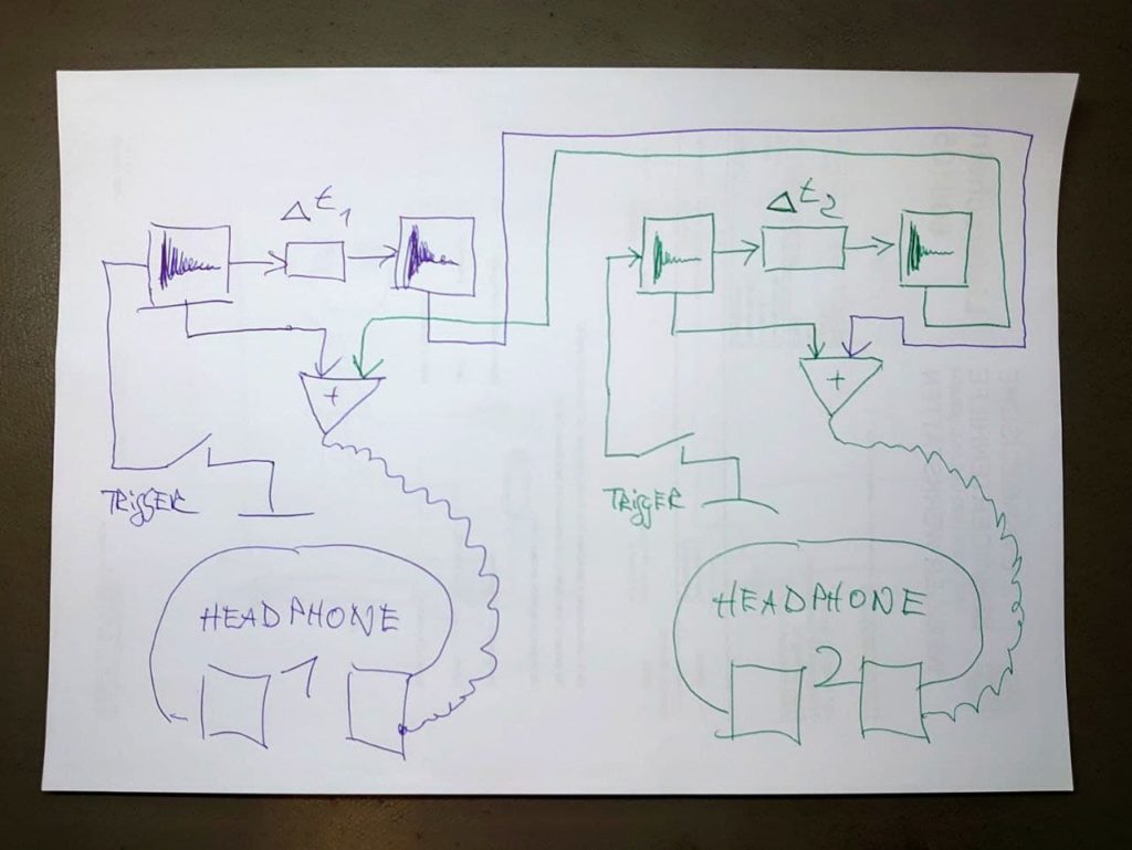

 denotes the instantaneous frequency, and
  the intrinsic frequency of oscillator
  , with
  .
.  denotes the coupling strength or sensitivity towards input signals to oscillator
  other oscillators in the network, as given by
  , the components of the adjacency matrix that are either one or zero depending on whether there is a connection from oscillator
  or not, respectively. The integral represents the signal processing or filtering within the feed-forward path of the oscillators, e.g., a low pass filter in a phase-locked loop oscillator with impulse response function
  .
.  denotes the phase of oscillator
  the transmission time delay for signals propagating from oscillator
  the feedback time delay within oscillator
  denotes the strength of the
  harmonic injection locking. Finally,
  denotes additive Gaussian white noise with variance
  .
. or
or  time delays, as the size of a system grows it becomes increasingly difficult to arrange the oscillators such that they can be coupled to any other in the network with the same transmission time delay; question: if there are transmission time delays that are heterogeneous within one connection (asymmetric), i.e., between an oscillator
  and
and 
 ?
? , for zero time delays
  , for identical oscillators
  ,
,  and for
  independently of the number of inputs we find
 radHz,
  radHz and simulate different network topologies, using simple MAX-CUT problems to benchmark. Note, that here the coupling strength
  (radHz)
 .
. oscillators, where oscillator
  receives input from all other oscillators while all other
  only receive from oscillator
  from that of oscillator

 realization for a fixed set of parameters and solve the MAX-CUT problem for a system of
  settles at a value of
  in that particular case, i.e., all phases have separated correctly. The
 the mean phase.
  if all oscillators are in-phase. In our benchmark case, all outer oscillators of the star topology form a subset that is shifted by a phase difference of
 for the particular MAX-CUT problem used for benchmarking here mentioned above and visible in Fig.~1.


 realizations shown in the plots were obtained for random initial conditions, choosing the initial phases of all oscillators as independent and identically distributed random variables from the interval
  . For some initial time we simulate the oscillators dynamics in the presence of noise and the SHIL perturbation with constant
  radHz to
  radHz, as shown in Fig. 9.
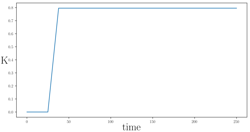
 oscillators align to one group and the other
  and ends at
  .
.
 . After free-running for few cycles the noisy oscillators with SHIL are coupled by linearly increasing the coupling strength
  , see Fig. 11.
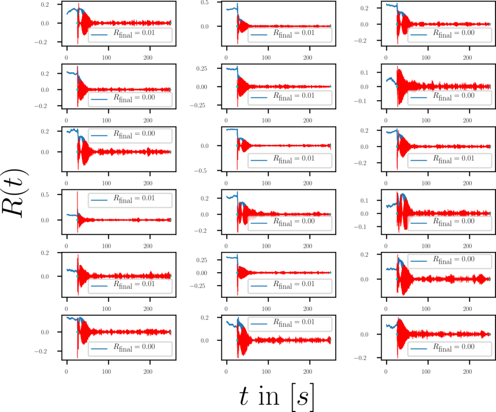
 (red) as a function of time. The final (mean) value of the order parameter is specified in the legend for each realization. The cyan diamonds represent the beginning and end of the measurement that is dedicated to measuring the time to solution.
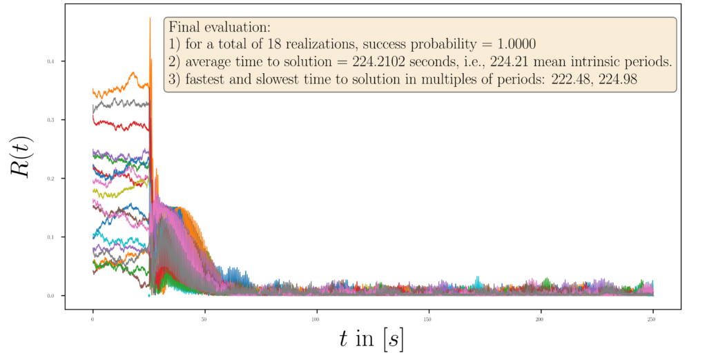
 , the slope of the linear ramp the network of mutually coupled oscillators solves the Maximum cut problem correctly with probability one.


 from independent identically distributed (
 ,
, and standard deviation
  . Note, that the two iid pseudo random numbers generated using the LTSpice rand()-function have to have different seed.
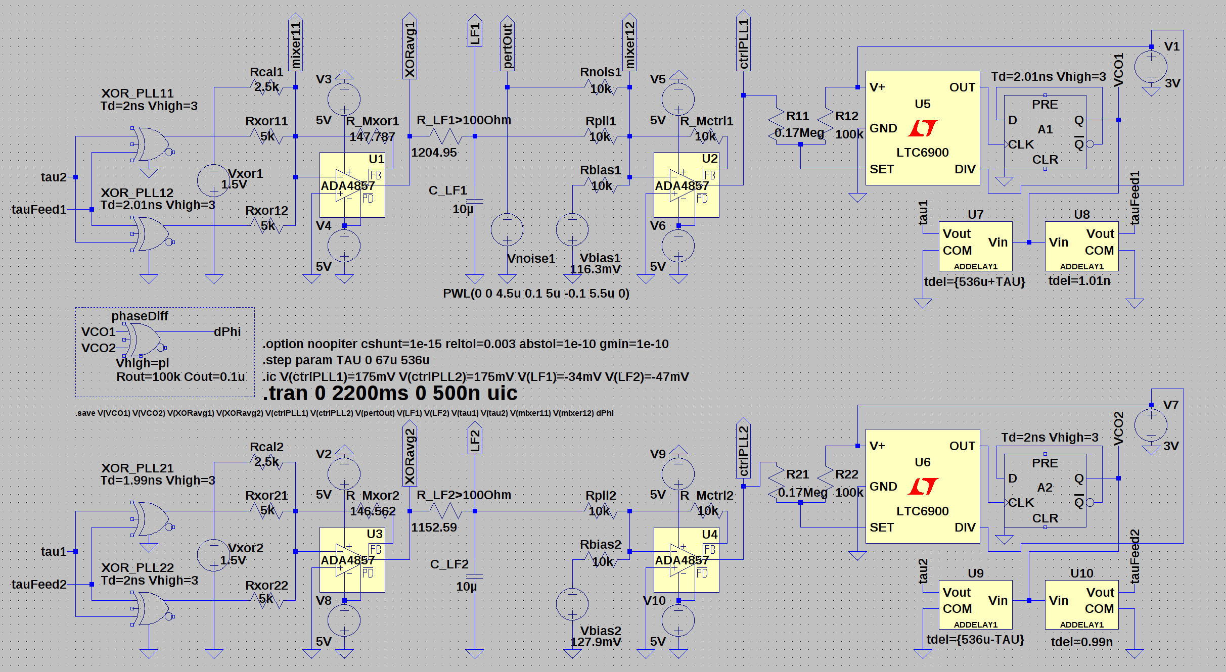
 mutually delay-coupled DPLL clocks running at a mean intrinsic frequency of
  MHz, see Fig. 1: LTspice block level circuit diagram of two delay-coupled DPLLs. Before that, we perform a separate SPICE simulation to measure the input response of the voltage-controlled oscillator, in this case a LTC6900, of our DPLLs. Hence we perform a parameter sweep transient simulations for each of which we change the input voltage to the LTC6900 VCO and measure the frequency of the output signal. We obtain the frequency from a Fourier analysis, using the FFT tool of the LTspice software. The result is shown in Fig. 2: VCO response curve. Note that we use a d-flip-flop at the output of the LTC6900 that divides the frequency by a factor two and ensures a
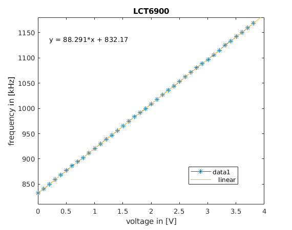
 MHz/V and the free running frequency
  MHz. As can be seen from the circuit diagram, the output signals of the two (here redundant) XOR phase detectors are mixed together with a shift voltage
  . The mixer is designed such that it takes into account all XOR outputs, that potentially originate from different coupling pairs, equally.
  . The offset signal can also shift the center frequency of the VCO, as will become clearer in the following. In the next step, we establish how the parameters of the SPICE circuit level simulations translate to the parameters of the phase model. With this we bridge the gap between these two abstraction layers. The phase model reads
![\begin{equation*} \dot{\phi}_k(t)=\omega_k+\frac{K_k}{n_k}\sum\limits_{l=1}^N\,\text{d}_{kl}\int\limits_0^{\infty}\text{d}u\,p_k(u)\,h\left[\phi_l(t-u-\tau_{kl})-\phi_k(t-u-\tau_{kl}^f) \right] \end{equation*}](https://lucas-wetzel.de/wp-content/ql-cache/quicklatex.com-561b237658c4465000232800361f5bb6_l3.png "Rendered by QuickLaTeX.com")
 denotes the instantaneous frequency,
  the impulse response of the loop filter,
  the feedback delay-time in the feedback path within PLL
 of the XOR output, and
  the scaling factor that scales the input sensitivity
  . In the circuitry this scaling is implemented by a
  and
and  .
.
 fF.
fF.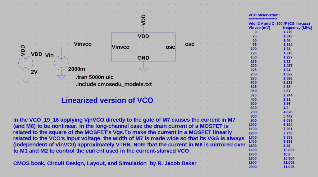
 .
.
 -twist or splay states.
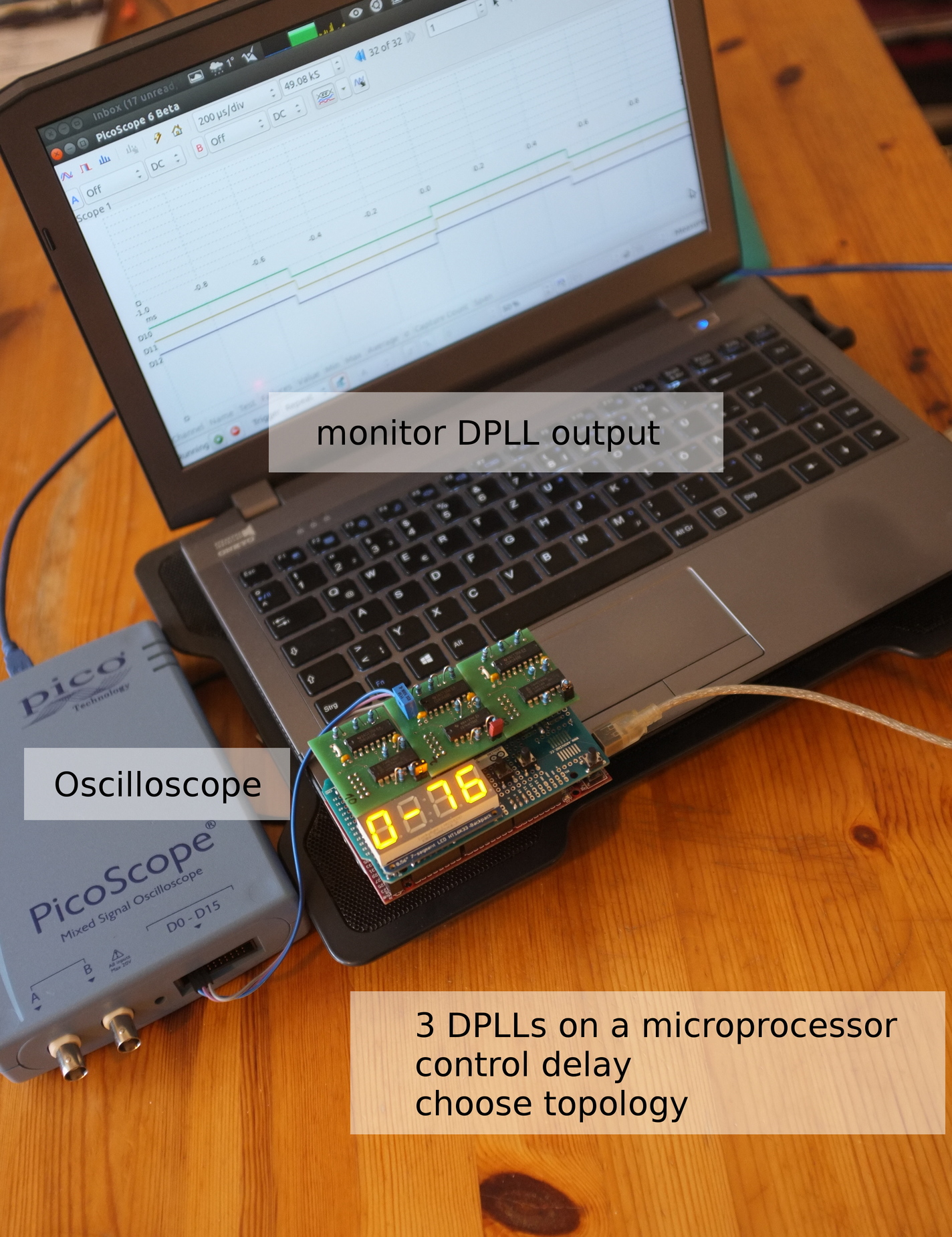
 s. Instead of using hundreds of kilometers of copper wiring, we use a micro-controller that buffers the states and histories of the PLLs and then sends these signals at specified delays to the respective coupled nodes in the clock network.
 square lattice with nearest neighbor interactions with open and closed boundary conditions.
 -adaption