Ising Machines based on networks of mutually coupled oscillators

Note, this is a work in progress, like a diary to formulate our thoughts and collect ideas, questions, hypothesis and results as we work towards gaining insight to the topic.

[collaborators: Dimitris Prousalis, Lucas Wetzel]

We want to thank Sven Köppel and Bernd Ulmann for their shared interest and the discussions.

Introduction

This post is about our exploration into the realm of so called Ising Machines. My curiosity into the topic was sparked by discussions with genius Bernd Ulmann, Mathematician, self-appointed Analog Evangelist, Inventor, Founder, museum director and most importantly a nice person.

An Ising machine is a physical implementation of a spin-system and its interactions to compute minima of the Ising Hamiltonian. As reviewed and shown, e.g., in “Ising formulations of many NP problems” by Andrew Lucas, many NP hard problems can be mapped onto the Ising Hamiltonian. Hence, if an Ising Machine can be build and scaled, it can act as an analog computer to solve these NP hard problems by finding/relaxing to ground states of the system. (Which is not guaranteed since the system may get trapped in a local minima. In this case some “shaking may help”.)

First of all I would like to link the first publications that I read to start with the topic. To be honest, they gave me a bit of a headache since by no means I was able to confirm the results that they presented when I stared looking at them in early 2021 — but more on that later. Here is the list to the open access manuscripts:

Hypotheses, issues and questions

When scaling Ising Machines to large numbers of spins (represented by oscillators whose phases are binarized) and to operate at high frequencies, the systems (spatial) dimensions may lead to non-negligible transmission time delays in the connections between the oscillators. We know, that such time delays can lead to multistability of in- and anti-phase synchronized states and therein. Furthermore, as the problem is usually encoded via the adjacency matrix of the network, these time delays will most likely be heterogeneous. Also, it has been shown that inert responses in, e.g., electronic oscillators, that stem from signal processing affect the self-organized dynamics in such systems.
The question is then, whether the mapping to the Ising Hamiltonian can still be justified and if not, which measures can be taken to achieve a sufficient (to solve a problem) approximation.
TODO: compile a list of open questions and problems related to the presence of time delayed coupling and inertia, quantify their effects in simulations and look for ways to address these.
When simulating delay-coupled phase oscillators using the Kuramoto model we made the following observations:
a) The results in Oscillator-based Ising Machine, chapter IV: Examples can be reproduced for sufficiently strong dynamical noise. If the noise was too small, we did not observe the convergence to the correct MAX-CUT solutions in all cases (actually we observed that only rarely). This could be a sign for rugged energy landscapes that require some ‘shaking’ to find the absolute minima and hence the correct solutions to the MAX-CUT problem.
b) When simulating using a second order Kuramoto model that takes into account inertia like effects introduced by, e.g., a loop filter in a phase-locked loop or the mass of a pendulum, the phases did not converge to the correct solutions for arbitrary loop filter cut-off frequencies. Increasing the cut-off frequency, or in other words, reducing the oscillators inert behavior, led again to the correct solutions. My hypothesis is, that loop filters with cut-off frequencies far below the second harmonic injection frequency will damped this too strongly and prevent he binarization of the oscillators phases. Hence, it may be beneficial to mix the second harmonic injection locking signal directly into the control signal of the PLL. In principle it may be possible to use a ‘copy’ of the feedback signal which is mixed with itself. The resulting output can then be filtered by a band-pass that allows only the second harmonic. These are however details the implementation of such an idea, in e.g., a PLL type of setup.
c) Adding small transmission delays seemed not to hinder convergence to the correct solutions, independently of whether the time delay would have led to in- or anti-phase synchronized states.

Notes for publication:

issues to be addressed: subharmonic injection locking in the presence of transmission delays that affect the frequencies of the oscillators – in that case the injection locking has to happen at roughly twice the instantaneous frequency of the oscillators
approaches discussed so far in the literature with electronic oscillators:
a) T. P. Xiao, Optoelectronics for refrigeration and analog circuits for combinatorial optimization, Ph.D. thesis, UC Berkeley (2019).
b) relaxation oscillators with capacitive coupling: A. Parihar, N. Shukla, M. Jerry, S. Datta, and A. Raychowdhury, Scientific reports 7, 1 (2017).
c) CMOS LC oscillators on chimera graph: N=240 in T. Wang, L. Wu, and J. Roychowdhury, in Proceedings of the 56th Annual Design Automation Conference 2019 (2019) pp. 1–2. and N=5 in J. Chou, S. Bramhavar, S. Ghosh, and W. Herzog, Scientific reports 9, 1 (2019).
d) RLC oscillators: LQ English, A. V. Zampetaki, K. P. Kalinin, N. G. Berloff, P. G. Kevrekidis, arXiv preprint arXiv:2204.00153

Playground, simulations & observations

Here I collect some results obtained from simulating different types of Kuramoto models. The code used here can be found on Github. The documentation process is still underway and I am being supported in cleaning up and organizing the code by Deborah Schmidt.

Along the results presented in Oscillator-based Ising Machine obtained by Matlab simulations of the Kuramoto model we start here and ask whether these results can be reproduced. Our model reads in the most general form [1,2,3]:

(1) $\begin{equation*} \begin{split} \dot{\theta}_k(t) = \omega_k &+ \frac{K_k}{n_k}\sum\limits_{l=1}^N\,d_{kl}\int\limits_0^\infty\,\text{d}u\,p(u)\,h\left(\theta_l(t-u-\tau_{lk})-\theta_k(t-u-\tau_{kl}^\textrm{f})\right) \\ &-K^\textrm{I}\int\limits_0^\infty\,\text{d}u\,p(u)\,h\left(2\,\theta_k(t-u-\tau_{kl}^\textrm{f})\right)+\sqrt{\sigma^2}\xi_k(t), \end{split} \end{equation*}$

where $\dot{\theta}_k(t)$ denotes the instantaneous frequency, and $\omega_k$ the intrinsic frequency of oscillator $k$ , with $k=1,\,\dots,\,N$ . $K_k$ denotes the coupling strength or sensitivity towards input signals to oscillator $k$ from $n_k$ other oscillators in the network, as given by $d_{kl}$ , the components of the adjacency matrix that are either one or zero depending on whether there is a connection from oscillator $k$ to $l$ or not, respectively. The integral represents the signal processing or filtering within the feed-forward path of the oscillators, e.g., a low pass filter in a phase-locked loop oscillator with impulse response function $p(u)$ . $\theta_k(t)$ denotes the phase of oscillator $k$ , $\tau_{lk}$ the transmission time delay for signals propagating from oscillator $l$ to $k$ , and $\tau_{kl}^\textrm{f}$ the feedback time delay within oscillator $k$ . $K^\textrm{I}$ denotes the strength of the $2^\textrm{nd}$ harmonic injection locking. Finally, $\xi_k(t)$ denotes additive Gaussian white noise with variance $\sigma^2$ .

In terms of the model, we aim to address how the following parameters affect finding the ground states and relate to the classical Ising model:

how to appropriately increase $K$ or $K^\textrm{I}$ , which one preferably and at what rate, does it depend on the network size?
the role of the loop filter via the $p(u)$ , the filter transfer function – if the cut-off frequency is below the $2^\textrm{nd}$ harmonic frequency, then the injection locking signal will be damped/filtered and binarization may be impaired (here we should consider a modified PLL architecture where the $2^\textrm{nd}$ harmonic injected signal does not pass trough the loop filter, e.g., multiplication by itself and band-pass to extract $2^\textrm{nd}$ harmonic)
the role of feedback $\tau_{kl}^\textrm{f}$ and transmission $\tau_{kl}$ time delays, as the size of a system grows it becomes increasingly difficult to arrange the oscillators such that they can be coupled to any other in the network with the same transmission time delay; question: if there are transmission time delays that are heterogeneous within one connection (asymmetric), i.e., between an oscillator $k$ and and oscillator $l$ , this leads to phase-difference between these oscillators for the case of pure mutual coupling without injection locking – how does that affect a networks ability to relax to a ground state of the Ising model? the same holds for the case $\tau_{kl}=\tau_{lk}$ and $\tau_{kl}\neq\tau_{k'l'}$
what about the coupling capacity/normalization of the inputs? does an oscillator couple more strongly the more inputs it receives?
should the coupling between the oscillators be repelling, i.e., should $K<0$ ?

Reproduce

When removing the loop filter $p(u)=\delta(u)$ , for zero time delays $\tau_{kl}^\textrm{f}=\tau_{kl}=0$ , for identical oscillators $\omega_k=\omega$ , $K_k=-K$ and for $n_k=1\,\,\forall\,\,k$ independently of the number of inputs we find

(2) $\begin{equation*} \begin{split} \dot{\theta}_k(t) = \omega - K\sum\limits_{l=1}^N\,d_{kl}\,h\left(\theta_l(t)-\theta_k(t)\right) -K^\textrm{I}\,h\left(2\,\theta_k(t)\right)+\sqrt{\sigma^2}\xi_k(t). \end{split} \end{equation*}$

In the publication Oscillator-based Ising Machine, see chapter IV, they set $K=5\,$ radHz, $K^\textrm{I}=2\,$ radHz and simulate different network topologies, using simple MAX-CUT problems to benchmark. Note, that here the coupling strength $K$ is increased linearly / ramped up once the simulation has started. We chose for the noise strength $\sigma^2=1E-3$ (radHz) $^2$ .
Using the same parameters we find the following results for a system of $N=20$ oscillators, where oscillator $k=1$ receives input from all other oscillators while all other $k=2,\,\dots,\,N$ only receive from oscillator $k=1$ . Hence, we have a star-like topology with oscillator $k=1$ being the center. In this case, the MAX-CUT problem is solved if all oscillators $k=2,\,\dots,\,N$ evolve to a phase different by $\pi$ from that of oscillator $k=1$ . The results were promising and lead to the correct solution of the MAX-CUT problem in most cases, however not in all cases as we show in the figures below:

(correct solution)

Fig. 1: Shows the frequency of all oscillators in the first row, the phase differences with respect to the phase of oscillator k=1 (dashed line) in the second row and the Kuramoto order parameter in the third row. Observe how the binarized phases of the oscillators separate successfully the nodes of the network into two groups according to the MAX-CUT of this network.

(incorrect solution)

Fig. 2: Shows the same plots as in Fig. 1 above. Observe how a few of the binarized phases of the oscillators do not separate to the correct subgroup and hence the MAX-CUT problem was not solved correctly. In this case we may have ramped up the coupling strength too quickly. This is an aspect that we will explore in more detail in the following.

We then realized the importance of the process of ramping up the coupling strength for finding the correct solution successfully. Also, adding dynamical frequency noise seemed to help convergence. Moreover, we simulated some realizations with time delay, signal filtering and ramping up the $2^\textrm{nd}$ harmonic injection coupling strength instead of the coupling strength of the first harmonic coupling terms. This had profound impact on whether the correct solution to the optimization problem was found. Therefore we decided to develop ideas on how to approach the impact of these parameters in a more structured way. Our preliminary results is what we will present in the following.

How we measure the success probability and time to solution as we change different system parameters?

We decided to run a number of $R$ realization for a fixed set of parameters and solve the MAX-CUT problem for a system of $N=20$ oscillators arranged in a star like topology, where an oscillator indexed by $k=1$ is located in the middle of the star and hence receives input from all others, while all others only receive input from $k=1$ , the center oscillator. After computing $R$ realizations we ask how many have led to a correct solution and in what average time that was achieved. A realization is categorized at being solved correctly when the magnitude of the order parameter $R(t)$ settles at a value of $0.9$ in that particular case, i.e., all phases have separated correctly. The Kuramoto order parameter is defined as

(3) $\begin{equation*} R(t)e^{-i\Psi(t)}=\frac{1}{N}\sum\limits_{l=1}^N\,e^{i\theta_l(t)}, \end{equation*}$

where $R(t)$ denotes the magnitude of the order parameter and $\Psi(t)$ the mean phase. $R(t)$ measures the synchrony of the oscillators and approaches $1$ if all oscillators are in-phase. In our benchmark case, all outer oscillators of the star topology form a subset that is shifted by a phase difference of $\pi$ with respect to oscillator $k=1$ . One can then calculate

(4) $\begin{equation*} R(t)=\sqrt{\left( \frac{1}{N}\sum\limits_{l=1}^N \cos(\theta_l(t)) \right)^2 + \left( \frac{1}{N}\sum\limits_{l=1}^N \sin(\theta_l(t)) \right)^2}, \end{equation*}$

which yields the result $R(t)=0.9$ for the particular MAX-CUT problem used for benchmarking here mentioned above and visible in Fig.~1.

A few more words on how we obtained the statistics on the realizations automatically from the simulations.
In order to determine whether the correct solution to MAX-CUT problem was found we checked the asymptotic values of the phase differences. Hence, if the phase differences of all oscillators $k=1,\,\dots,\,N$ with respect to the phase of $k=1$ are equal to $\pi$ asymptotically, the correct solution has been obtained. We quantify this by checking these phase-differences and the value of the order parameter. Since the phase-configuration should be constant once the system has settled to the ground state, we compute the average over one and a half period of the intrinsic oscillations of the oscillators.
Extracting the mean time until a solution is obtained is measured as follows. We consider only those realizations that led to a correct solution of the MAX-CUT problem. For these, we calculate the time-derivative of the order parameter which we then average over half a period of the intrinsic frequency of the oscillators. This yields a more smooth curve. We then track from the end of the time-series towards the beginning, i.e., backwards in time, when the order parameter changes for the first time. This represents the end of the transient dynamics that led to the solution. To calculate the time to solution, we choose the difference between the time when the transient dynamics have finished and the time where we started to ramp up the coupling strength.

Here is an example how the resulting plots look like:

Fig. 3: Kuramoto order parameters for all 18 realizations as a function of time in one plot. The blue dots at R(t)=0 mark the points between which we measure the time to solution for correct solutions. The text box shows the statistics, i.e., the percentage of realizations that led to the correct solution and the average time that this required.

Fig. 4: All Kuramoto order parameters (blue) and their time derivative (red) for all realizations as a function of time in individual plots. The blue dots at R(t)=0 mark the points between which we measure the time to solution for correct solutions. The text box shows the asymptotic value of the order parameter.

Fig. 5: Time series of all phase differences with respect to the phase of oscillator k=1 (dashed line). Initially the phases were distributed between -pi and pi, here they are plotted between -pi/2 to 3pi/2. In that case in- and anti-phase synced states are clearly visible without noise induced slips at the modulo boundary. All realizations show the correct solution to the MAX-CUT problem.

Fig. 6: Time series of the output signals of all oscillators, here digital, plotted for each realization individually.

Results for networks of oscillators that respond instantaneously and where no transmission time delays are present

In a network of $N=20$ mutually coupled oscillators with second harmonic injection locking (SHIL) we show that the Maximum cut problem can be reliably solved. The oscillators have an infinite modulation bandwidth and there are not time delays associated to the mutual coupling between the oscillator nodes of the network. We benchmark with the network topology shown in Fig. 7.

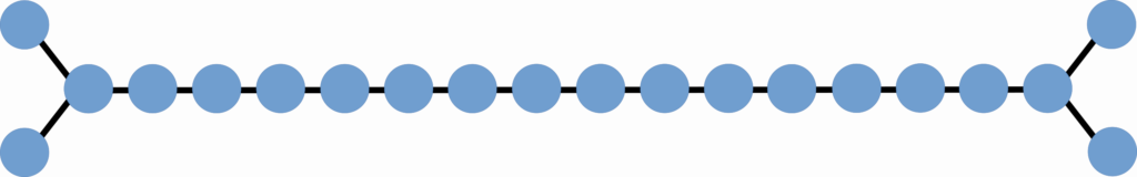
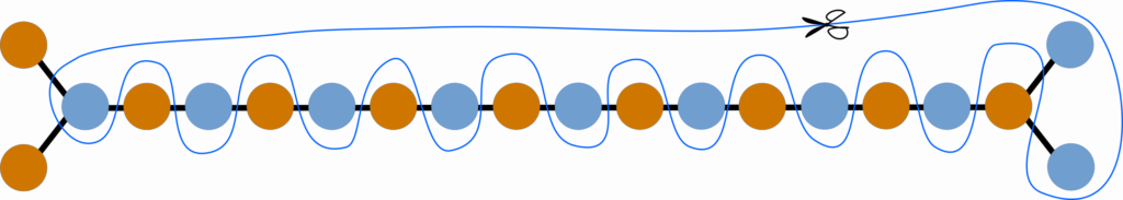
Fig. 7: Network topology used to benchmark the MAX cut problem with equal edge weights.

The correct MAX cut solution to this problem looks as shown in Fig. 8, where the different colors separate the two populations of nodes defined by the Maximum cut.

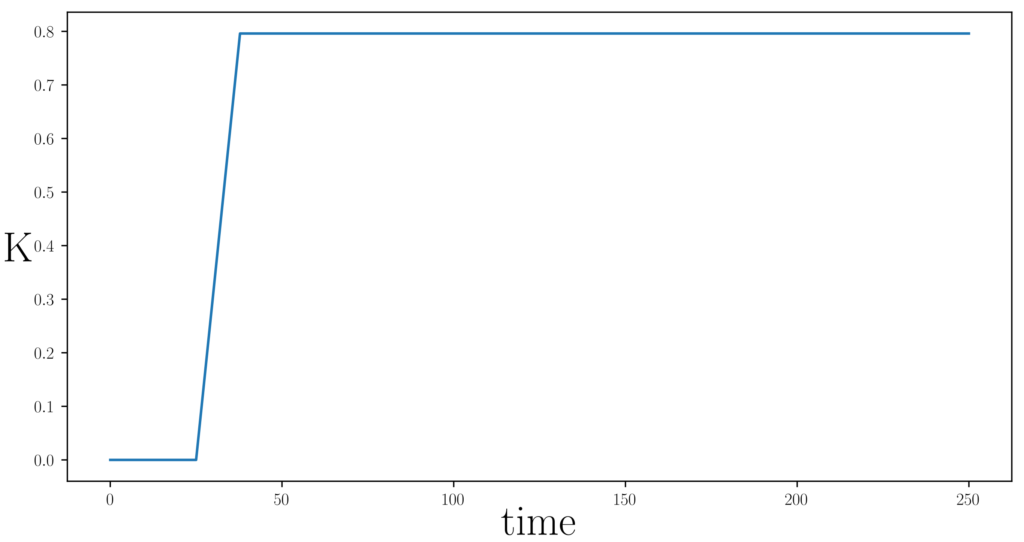
Fig. 8: Maximum cut solution to the network topology shown in Fig. 7.

The result of the $18$ realizations shown in the plots were obtained for random initial conditions, choosing the initial phases of all oscillators as independent and identically distributed random variables from the interval $[-\pi,\,\pi)$ . For some initial time we simulate the oscillators dynamics in the presence of noise and the SHIL perturbation with constant $K^\textrm{I}=2\,$ radHz. Then we ramp up the coupling strength $K$ of the mutual interaction terms from $K^\textrm{init}=0$ radHz to $K^\textrm{final}=2\,pi\,0.8$ radHz, as shown in Fig. 9.

Fig. 9: Time dependence of coupling strength $K$ of the mutual coupling between the oscillators in Hz/[Volt].

Given the ‘ground truth’ above, we hence expect that $10$ oscillators align to one group and the other $10$ to the group that is separated by $\pi$ from the first. The order parameter $R(t)$ is then expected to be equal to zero. Here we show the plots of the phase differences with respect to the first oscillator in the system, see Fig. 10. Note that in the plots the oscillator numbering starts from $0$ and ends at $N-1$ .

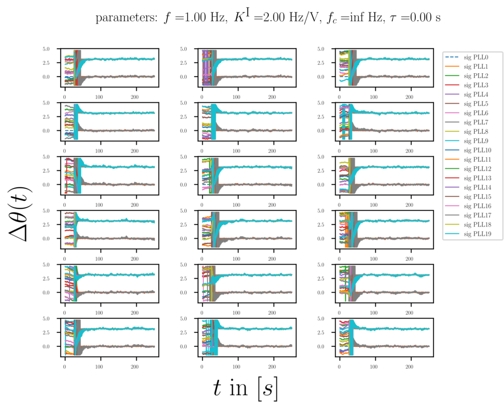
Fig. 10: Phase differences of all oscillators with respect to oscillator $k=0$ . After free-running for few cycles the noisy oscillators with SHIL are coupled by linearly increasing the coupling strength $K$ , see Fig. 9 and two populations with distinct phase differences form.

The order parameter plots associated to the phase difference plots in Fig. 10 reveal that there are indeed two populations with $10$ oscillators in each. The populations are separated by a phase-difference $\pi$ and hence the order parameter $R(t)=0$ , see Fig. 11.

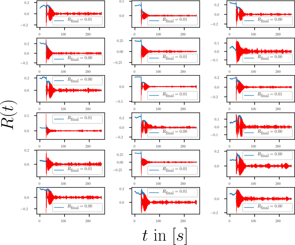Fig. 11: The order parameter $R(t)$ (blue) and its time derivative $\dot{R}(t)$ (red) as a function of time. The final (mean) value of the order parameter is specified in the legend for each realization. The cyan diamonds represent the beginning and end of the measurement that is dedicated to measuring the time to solution.

An overview plot of all the order parameters for all realizations and the ‘statistics’ (it’s only 18 realizations) concludes that all cases were solved correctly by the relaxation dynamics, see Fig. 12. Note that the automatized measurement of the relaxation time, i.e., the time to solution failed here due to the fluctuations of the order parameter. This feature will be reworked in the next iteration.

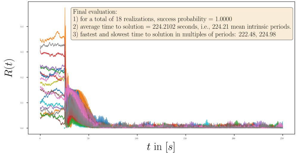Fig. 12: All order parameters $R(t)$ for all realizations. Note that due to the fluctuations of the order parameter the automatic estimation of the time to solution FAILED. From inspection by eye we estimate an average time to solution of about 30-50 periods of the intrinsic frequency.

Hence we have to rework the way the automatic estimation of the time to solution is performed. We will use smoothing functions in the future to obtain a moving average that accounts for boundary effects. These results show that with the right choice of parameters $K$ , $K^\textrm{I}$ , and $r_K(t)$ , the slope of the linear ramp the network of mutually coupled oscillators solves the Maximum cut problem correctly with probability one.

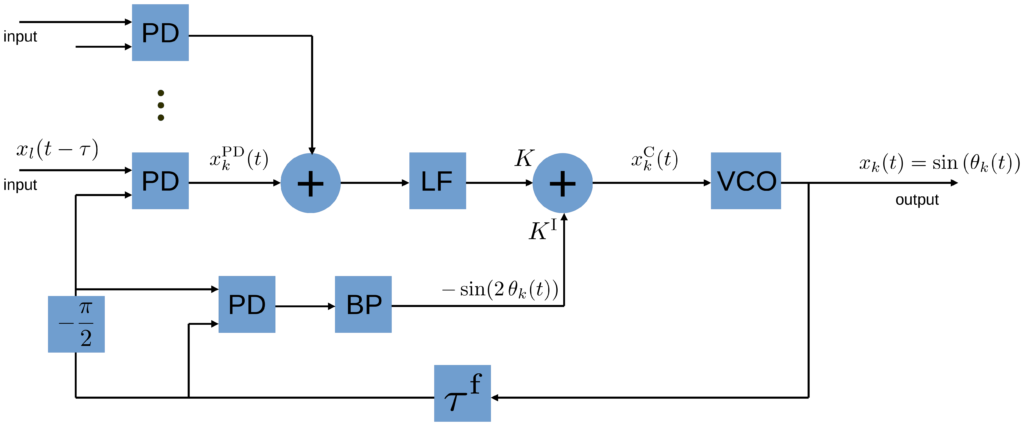
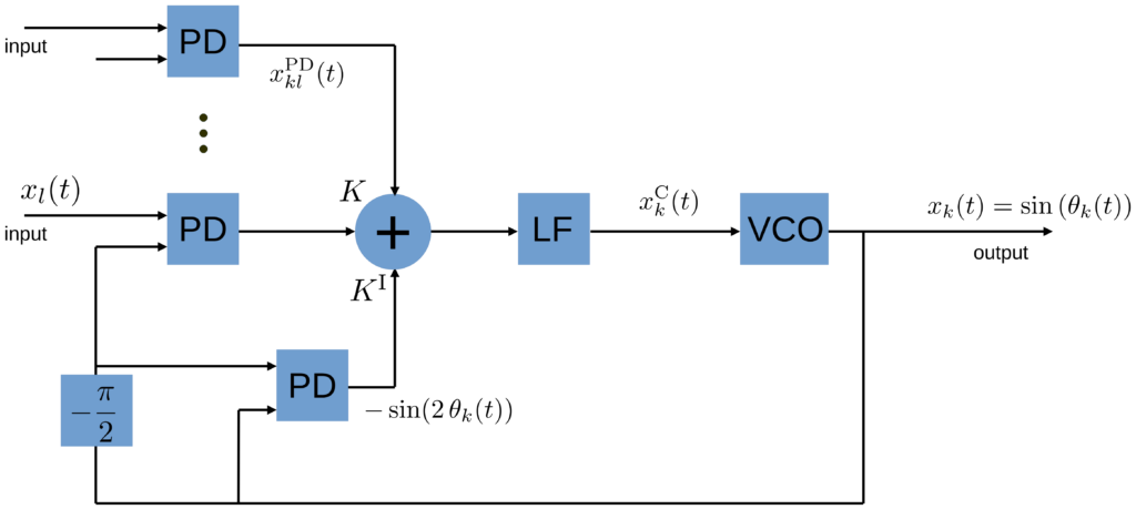
The results shown so far correspond to the following architecture design schematic of an oscillator with SHIL, see next Fig. XY.

Fig. XY: Schematic of a PLL with SHIL. There are no time delays in the network.

Adding inert oscillator responses

In that case we obtain the following set of dynamical equations

(5) $\begin{equation*} \begin{split} \dot{\theta}_k(t) = \omega_k &+ \frac{K_k}{n_k}\sum\limits_{l=1}^N\,d_{kl}\int\limits_0^\infty\,\text{d}u\,p(u)\,h\left(\theta_l(t-u)-\theta_k(t-u)\right) \\ &-K^\textrm{I}\int\limits_0^\infty\,\text{d}u\,p(u)\,h\left(2\,\theta_k(t-u)\right)+\sqrt{\sigma^2}\xi_k(t), \end{split} \end{equation*}$

where the same notation holds as provided following Eq. (1). Note that in the case presented here, the SHIL signal is also filtered by the LF that filters the cross-coupling signals between the oscillators, see schematic Fig. XY1. This is an architecture design choice. We will later also discuss the case where the SHIL signal is added after the LF and is not filtered by the low pass.

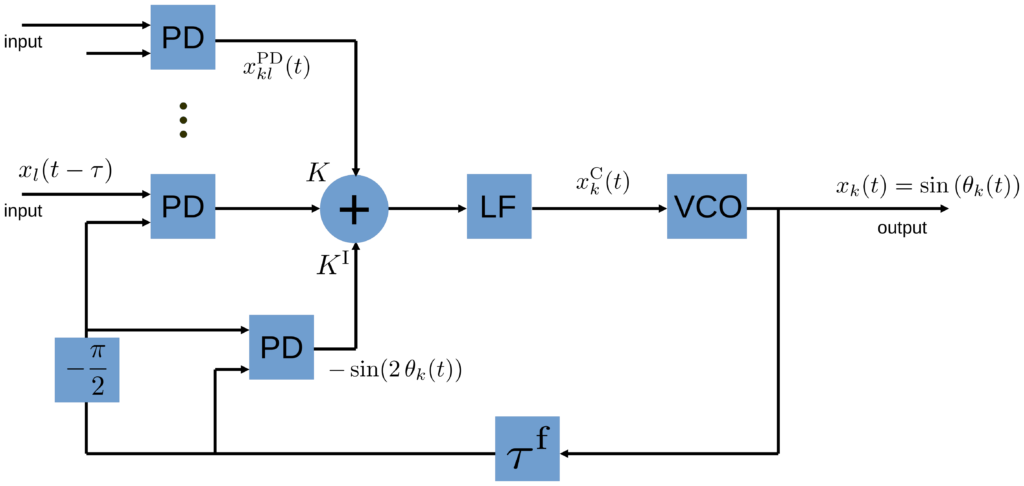
Fig. XY1: Schematic of a PLL with SHIL. The SHIL signal and the cross-coupling signals are filtered by the low-pass filter (LF).

Adding inert oscillator responses and transmission time delay

In that case we obtain the following set of dynamical equations

(6) $\begin{equation*} \begin{split} \dot{\theta}_k(t) = \omega_k &+ \frac{K_k}{n_k}\sum\limits_{l=1}^N\,d_{kl}\int\limits_0^\infty\,\text{d}u\,p(u)\,h\left(\theta_l(t-u-\tau_{lk})-\theta_k(t-u-\tau_{kl}^\textrm{f})\right) \\ &-K^\textrm{I}\int\limits_0^\infty\,\text{d}u\,p(u)\,h\left(2\,\theta_k(t-u-\tau_{kl}^\textrm{f})\right)+\sqrt{\sigma^2}\xi_k(t), \end{split} \end{equation*}$

where the same notation holds as provided following Eq. (1). Note that also in the case presented here, the SHIL signal is also filtered by the LF that filters the cross-coupling signals between the oscillators, see schematic Fig. XY2. This is an architecture design choice. We will later also discuss the case where the SHIL signal is added after the LF and is not filtered by the low pass.

Fig. XY2: Schematic of a PLL with SHIL. The SHIL signal and the cross-coupling signals are filtered by the low-pass filter (LF). The external signals and the feedback signal can be time-delayed.

Inert oscillator responses, transmission time delay and no LF filtering of the SHIL signal

In this case the SHIL signal is not fed through the LF together with the cross-coupling signals, however instead there is a band-pass filter that ensures that only the second harmonic contributions from the self-mixing of the oscillators passes to the control signal, see Fig. XY3.

Ising Machines based on networks of mutually coupled oscillators

Introduction

Hypotheses, issues and questions

Notes for publication:

Playground, simulations & observations

Reproduce

How we measure the success probability and time to solution as we change different system parameters?

Results for networks of oscillators that respond instantaneously and where no transmission time delays are present

Adding inert oscillator responses

Adding inert oscillator responses and transmission time delay

Inert oscillator responses, transmission time delay and no LF filtering of the SHIL signal

Leave a Reply Cancel reply